

Why did the old Folly end now, and no later? Why did the modern Wisdom begin now, and no sooner?
-Rabelais, Prologue to Book V
=======================
Academia, like our nation's morals, seems to be forever in peril. When I first heard of the replication crisis - about how standards are so loose that a scientist can't even replicate what he ate for breakfast three days ago, much less reproduce another scientist's experiment - I was reminded of my grandpa. He once complained to me that colleges today are fleshpots of hedonism and easy sex. Nonsense, I said. Each year literally tens of students graduate with their virtue intact.
Nonetheless, the more I learned about the replication crisis, the more alarmed I became. You know a crisis is serious when it has its own Wikipedia page, and when its sister phrase "questionable research practices" gets its own acronym: QRP (pronounced "Quirp"). These practices range from data "peeking" - ogling a p-value before she's half-dressed - to fabricating data, one of academia's gravest sins. (Apparently grant agencies have gotten very picky about researchers lying about their results and wasting millions of dollars.) One of my friends suggested campaigning for a War on QRPs, with scientists in white labcoats stamping out QRPs like cockroaches. Who knows - someday QRP Exterminator may become as respected and honorable a position as Lab Manager.
One such QRP was recently flushed out of hiding in an article by Eklund and colleagues published in the journal PNAS (pronounced "P-NAS"), with the klieg lights thrown on cluster correction, the most common FMRI multiple comparison technique. If you're in a neuroimaging lab, or if you've read about FMRI in a magazine, you've come across these clusters - splotches of reds and yellows, color-coded to show the strength of the result. They look attractive, especially on glossy magazine pages, and they make for good copy.
 |
| Relative popularity of different correction methods. The majority use cluster correction; a smaller percentage use voxel-based thresholding (i.e., correcting for the total number of voxels in the brain); and the remainder do not use correction. Men who don't use correction claim that it feels more spontaneous and natural. Adapted from Woo et al. (2014) |
There is another reason for the popularity of clusters: As each FMRI dataset contains tens or hundreds of thousands of voxels, and as each voxel is similar to its neighbor, it is useful to test whether a cluster of voxels is significant instead of each voxel individually. This increases the sensitivity of detecting activation, although at the cost of reduced spatial sensitivity. If I point to a cloud of smoke in the distance you will assume there is a fire somewhere, although seeing the cloud itself gives you only a vague idea of where or how big the fire is - or, for that matter, whether its the result of a dozen individual campfires, or of a single inferno.
Problems with Cluster Correction
The authors don't take issue with cluster correction per se; rather, they claim that the assumptions behind the technique, and how the correction is used, can lead to inflated false positives. In other words, using cluster correction makes one more likely to say that a cluster represents a true activation, when the cluster is actually noise. The assumptions they question are:
1) That spatial smoothness is constant over the brain; and
2) That spatial autocorrelation looks like a Gaussian distribution.
Spatial smoothness is in fact not constant; it varies over the brain. Midline regions such as the precuneus, anterior cingulate cortex, and prefrontal areas show more spatial smoothness than the the outer regions - possibly because the midline areas of cortex, with the gray matter of the hemispheres in close proximity to each other, have similar structure and similar timecourses of activity which are averaged together. The underestimation of spatial smoothness in these areas can lead to inflated false positives, which may be why midline areas (such as the anterior cingulate cortex) turn up as a significant result much more often than other areas.
 |
| Effects of spatial smoothing at different smoothing sizes, or kernels. The larger the smoothing kernel, the more that adjacent voxels are blurred together, resulting in greater similarity of spatial structure and also of the timecourse of activity. |
It is the second assumption, however, which is the main cause behind the increase in false positives demonstrated in the Eklund paper. The idea behind spatial autocorrelation is simple: A voxel is more similar to its immediate neighbors and less similar to voxels farther away, the similarity falling off in concentric spheres around a given voxel. This correlation between each voxel and its neighbors is traditionally modeled with a Gaussian distribution - the same bell-shaped curve that models most distributions, such as IQ or height - when in reality the autocorrelation distribution has much thicker tails:
 |
| Comparison of the Gaussian distribution (green) with the empirical ACF (black) and mixed model of a Gaussian and exponential distribution (red). Note the increasing discrepancy between the Gaussian distribution and the empirical distribution around 5mm, with the thicker tails of the empirical distribution suggesting that more distant voxels are more correlated than is assumed under traditional clustering methods. |
When the authors ran simulations on large datasets under different experimental conditions (e.g., block design and event-related), they found that this assumption of a Gaussian shape led to false positives far above the expected 5% rate across all the major software packages (SPM, AFNI, and FSL). The commonly used p = 0.01 threshold for the individual voxels of the cluster led to much higher false positive rates than a more stringent p = 0.001 threshold. (Notably, permutation testing, a nonparametric method that does not rely on assumptions of normality, did not show any substantial difference in false positives under any conditions.) These inflated false positive rates led to the following figure, which was picked up by the popular media and discussed in a fair, evenhanded way which emphasized that although false positive rates could be increased in some cases, it would be hasty to conclude that all neuroimaging results are wrong.*
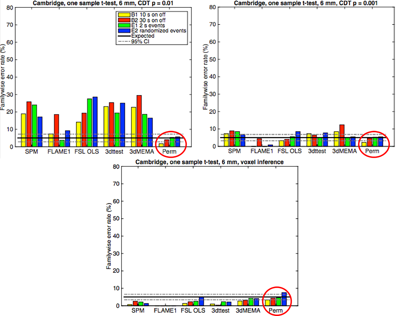 |
| Figure 1 from Eklund et al (2016). Simulations on an open-access dataset for different block and event-related designs. Upper left: Cluster-defining threshold (CDT) of p = 0.01 uncorrected; upper right: CDT of p = 0.001 uncorrected; bottom: voxel-level inference. Black line: Expected false positive rate of 5%. A threshold of p = 0.01 leads to inflated false positives across all of the major software packages (SPM, AFNI, and FSL), while a threshold of p = 0.001 leads to clusters closer to the expected 5% false positive rate. Voxel-level inference is slightly conservative in all cases. Permutation testing (circled in red), a nonparametric method, does as expected under all conditions. |
*Or not.
Solutions
There are three solutions to this problem; solutions to make neuroimaging respectable again, to cease being laughed at as cranks, charlatans, raiders of the public fisc, and attention-seeking, unscrupulous bloggers.
One solution is to use voxel-wise thresholds; although, as shown in the Eklund paper, these are often far too conservative, and can lead one to conclude there are no results when they actually do exist. I, for one, cannot stand the thought of those poor results slowly suffocating in their little gray coffins, alive but unable to signal for help. With voxel-wise thresholds we stop up our ears with wax; we think we hear the dim scratching of nails, the whimpers for succor, but dismiss them as figments of a fevered imagination; and we leave those tiny blobs and their tiny blob families to know that their last moments will be horror.
The second, more humane solution is to use more conservative cluster-forming thresholds, such as p = 0.001 uncorrected, in conjunction with more accurate modeling of the spatial autocorrelation. I recommend updating your AFNI binaries to the latest version (i.e., the beginning of 2017 or later), and using the -acf option in 3dFWHMx. For example:
3dFWHMx -mask mask+tlrc.HEAD -acf tmp.txt errts+tlrc.HEAD
Which will generate parameters for a more accurate estimation of the empirical ACF; you will see something like this:
++start ACF calculations out to radius = 37.68mm
+ACF done (0.74 CPU s thus far)
11.8132 13.748 12.207 12.5629
0.260939 6.36019 16.6387 19.1419
The first line of numbers are the traditional smoothness estimates in the x-, y-, and z-directions, as well as a weighted average of them (bolded). The second line of numbers are the a, b, and c parameters for the ACF model,
a^(-r*r/(2*b*b))+(1-a)^(-r/c)
With the last number being an updated estimate of the smoothness. These are then input into 3dClustSim:
3dClustSim -acf 0.26 6.36 16.64 -mask mask+tlrc.HEAD -athr 0.05 -pthr 0.001
The difference between the two smoothness estimates leads to substantial differences in significant cluster thresholds. In this case, the traditional estimates lead to a cluster threshold of 668 contiguous voxels, while the ACF version gives a threshold of 1513. This was using an initial cluster-defining threshold of p = 0.01, which can lead to such large differences; more stringent thresholds (e.g., p = 0.001) have less of a difference, but still a significant gap between them.
The third solution is to use non-parametric methods, such as permutation tests; which, since they do not rely on assumptions of normality, are immune to the autocorrelation assumptions listed above. Some popular tools include SPM's SnPM (Statistical non-Parametric Mapping); FSL's randomise; and Eklund's BROCCOLI. Out of the three, I've only used randomise, and found it straightforward to use (see the tutorial here).
Conclusions
Have we been profiting too long from dubious methods in neuroimaging? Have we become lax and complacent in our position as a period science, knowing that no matter how poorly designed the experiment is, no matter how ludicrous the question we are investigating - such as where the word YOLO is in the brain, or how the consumption of Four Loko affects delayed discounting - no matter whether our subjects are technically alive or not, we will probably still get a significant result, most likely in the precuneus?**
The answer to all of these, I would say, is yes. But just because I was able to get the results of my first paper to squeak by with an outdated version of AlphaSim, and consequently have an easy time in graduate school, make tons of money, and be envied by all of my friends, doesn't mean that you should have the same privilege. The way forward will be a hard one for the neuroimagers of today; standards will be higher, methods tighter, reviews harsher. But if you put in enough work, if you exercise enough diligence, and if you live long enough into the ninth year of your graduate program, you may just be able to take advantage of the next major statistical loophole that comes along. Have faith.***
**For the record, I still don't know where the precuneus is. My best guess is: "Somewhere right before the cuneus."
***In all seriousness, AFNI has been responsive, helpful, and, given the circumstances, even gracious with any issues that have come up with their programs - specifically, 3dFWHMx (the smoothness estimator) and 3dClustSim (the cluster threshold estimator). The problems are not so much with AFNI, as with how it is used; and even though it is being patched, it is worth keeping in mind that there will likely be other issues discovered in the future, as with all methods - even non-parametric ones. (Their response to the Eklund paper can be found here.) The responsibility of the user is to make sure that the results that are reported follow the most up-to-date correction methods; that suspicious-looking activations that don't make sense in the experimental context, or consist of several blobs connected by threads of voxels, should be interpreted with caveats; and that even results which are weak and do not pass correction with the current methods, may still be real but underpowered effects. As with any result, it's up to the researcher to use their best judgment.
Hello Andy, Thank you for these interesting comment. Not centrally related to the topic, but I found the template you use at the top is terrific. Would you mind sharing whether this can be access through SPM or similar to map own results?
ReplyDeleteThanks
P
Hey Pablo, the template is from the program SurfIce, which you can find here: https://www.nitrc.org/projects/surfice/
DeleteGive it a spin and see how it goes!
-Andy
Hi Andy,
ReplyDeleteI've done all my analyses in SPM8, but I'd like to use 3dClustSim for cluster level correction. Wondering if instead of using AFNI's 3dFWHM to get estimates of the smoothness, can I use the effective smoothness values listed at the bottom of the results file from my SPM.mat? Or are those the "traditional" smoothness values you mention and I've missed the point of doing the -acf? If you recommend using 3dFWHM function, can you tell me what these inputs refer to please if I have files generated via SPM (I"m brand new to AFNI and plan on learning more soon!). 3dFWHMx -mask mask+tlrc.HEAD -acf tmp.txt errts+tlrc.HEAD
Thank you so much for your helpful blog and videos!
Best,
Val
Hi Val,
DeleteApologies for the late reply! Yes, you should be able to use 3dFWHMx on the residuals of the SPM data. I wouldn't use the estimated FWHMx values you see at the bottom of the SPM results window, as they probably underestimate the true smoothness of the data.
If you want to use AFNI's 3dFWHMx, here's what the options refer to (and what they correspond to in the SPM dataset, surrounded by brackets):
-mask [mask.nii]: Refers to a mask covering the whole brain and excluding non-brain material (e.g., air)
-acf tmp.txt: Computes the autocorrelation function that fits an updated model of the smoothness (you can actually omit the tmp.txt part, I'm not sure what the output in the tmp.txt file means)
errts+tlrc.HEAD [ResMS.nii]: Refers to the residual time series (although in SPM, this is a single volume, not a time series; and it is the mean square of the residuals, not the residuals themselves)
Note that there's another option in 3dFWHMx called 2difMAD, which is used for single-volume residual datasets (such as PET images). It might be applicable in this case since the ResMS.nii image is a single volume, but in my experience the difference is negligible between including the 2dMAD option and omitting it.
Here's what I would recommend:
1. Calculate the square root of the ResMS.nii image to "undo" the mean square scaling of the residuals: 3dcalc -a ResMS.nii -expr 'sqrt(a)' -prefix MS.nii
2. Use this MS.nii dataset to estimate your FWHMx: 3dFWHMx -acf -mask mask.nii MS.nii
3. Use the second row of the ACF output with 3dClustSim to estimate your updated clusters.
Again, I'm not 100% sure about this entire procedure - for example, taking the square root of the ResMS.nii dataset. But in my simulations it provided smoothness estimates that were comparable to what I had seen when analyzing AFNI data with similar smoothing kernels.
Good luck!
-Andy
Thanks Andy!! Less daunting than re-doing all the first levels to get residuals for ~260 scans, for sure. I will give this a shot! :) - Val
Delete[EDIT 03.26.2019]: Using ResMS.nii is probably NOT appropriate for estimating the smoothness of the data; instead, I recommend saving out the residuals during the “Estimate” stage of the analysis. When you press the Estimate button in SPM there is an option for writing out the Residuals, which by default is set to No. Change this to Yes, concatenate the timeseries using a command like fslmerge or 3dTcat, and then run 3dFWHMx on that dataset.
DeleteMy previous comments were based more liberal cluster-defining thresholds such as p=0.05, which seemed to give comparable cluster size estimates when using either SPM’s ResMS.nii or AFNI’s errts+tlrc. At lower thresholds such as p=0.001, the cluster sizes appear to differ dramatically. I would therefore recommend either running your model estimation in AFNI and using the errts+tlrc file for smoothness estimation, or using the residuals output by SPM.
Hi Andy!
ReplyDeleteThank you for all the information that you share.
I have a question regarding 3dClustSim. Actually, I dont understand well the output.
So, the output of 3dClustSim is a table with phrt/alpha and cluster size. Does this mean that any cluster size with a significant alpha value is significant?
For example, I perform a 3dMEMA (comparing two groups) and I run 3dClustSim. the output is the table below. if I chose an alpha & phrt value of 0.05, the cluster size is, 7.3. Then, does this mean that any cluster sized 7.3 (in my 3dMEMA comparison A vs B) is significant?
Thank you!
CLUSTER SIZE THRESHOLD(pthr,alpha) in Voxels
# -NN 1 | alpha = Prob(Cluster >= given size)
# pthr | .10000 .09000 .08000 .07000 .06000 .05000 .04000 .03000 .02000 .01000
# ------ | ------ ------ ------ ------ ------ ------ ------ ------ ------ ------
0.100000 10.4 10.5 10.7 10.8 11.0 11.1 11.3 11.6 12.0 12.6
0.090000 9.7 9.8 9.9 10.0 10.2 10.3 10.5 10.8 11.2 11.7
0.080000 8.9 9.0 9.1 9.2 9.4 9.5 9.7 10.0 10.3 10.9
0.070000 8.2 8.3 8.4 8.5 8.6 8.7 8.9 9.1 9.4 10.0
0.060000 7.5 7.6 7.6 7.7 7.9 8.0 8.1 8.3 8.6 9.0
0.050000 6.8 6.8 6.9 7.0 7.1 7.2 7.3 7.5 7.8 8.2
Hi Myriam,
DeleteYes, that is how you can interpret the table: According to the simulations, due to chance you would expect to see 5% of the time a cluster of 7.3 voxels all individually passing 0.05. Round this up to 8 voxels to make sure that you are controlling for a 5% false-positive rate.
However, those voxel numbers look very low to me; are you using a mask for small volume correction? Also, are you using the FWHM estimates from FWHMx? For 0.05, they should be very stringent, and usually large enough to remove any clusters with any spatial specificity, which is why most people use cluster-forming thresholds of 0.01 or 0.001 nowadays.
-Andy
Hello Andy,
ReplyDeleteI have a question. So I did 3dClustersim and then I took alpha(athr)=0.05 and pthr=0.001 and the #voxels was like 22 for a certain correlation mapping, and when I tried to see how it looks,it didnt show me anything, so I increased the pthr to 0.05 same as athr, and got more number of voxels, and was able to see clearly the cluster portion. now does this pthr mean the same like my results are statistically significant when pvalue is <= alpha? but in here, 0.001 is much less than 0.05 so I should consider 0.001 results as more significant than pvalue being 0.05. I am kind of confused, as that exactly is this pthr and athr with respect to statistical analysis?