Showing posts with label fMRI. Show all posts

Friday, March 31, 2017

NIH Talk: Distinct Regions of mPFC Process Pain and Cognition


Grown-ups like numbers. When you tell them about a new friend, they never ask: "What does his voice sound like?" "What games does he like best?" "Does he collect butterflies?" They ask: "How old is he?" "How many brothers does he have?" "How much does he weigh?" "How much does his father make?" Only then do they think they know him. If you tell grown-ups, "I saw a beautiful red brick house, with geraniums at the windows and doves on the roof..." they won't be able to imagine such a house. You have to tell them, "I saw a house worth a hundred thousand francs." Then they exclaim, "What a pretty house!"

--Saint-Exupery, The Little Prince


I often have vivid fantasies about how my talks will be received: The audience will laugh at my jokes; listen in attentive silence about the obstacles I overcame to carry out my research; gasp in astonishment as I reveal my big finding which will change the field forever. And, at the end of my talk - concluded with a germane and heartfelt anecdote which ties everything together - an ocean-like roar of applause and yells as I am lifted up high on a chair and carried through the streets with great honor. The men shake my hand vigorously and the ladies kiss me on the cheek. "Hats off, gentlemen!" says the town crier, "A genius!"

For some reason, and much to my dismay, reality fails to match my heart's desires. The jokes and asides feel flat and fall stillborn from my mouth. The background of my study feels less like an epic and more like reciting a laundry list. (I swear it sounded much more interesting when I was rehearsing it to myself.) Any small issue with the projector cutting out or with my Powerpoint animations failing to work, in the moment feels as embarrassing and indecent as being caught with my fly unzipped.

But I keep going nonetheless, holding out hope to someday achieve that perfect talk combined with the perfect moment. The ultimate trade awaiting the ultimate practitioner.

In any case, something to strive for.

Tuesday, March 28, 2017

Video Introduction to ROI Analyses


About forty years ago certain persons went up to Laputa, either upon business or diversion, and upon their return began to dislike the management of everything below, and fell into schemes of putting all arts, sciences, languages, and mechanics upon a new foot. To this end they procured a royal patent for erecting an Academy of Projectors in Lagado. Every room hath in it one or more projectors. The first man I saw had been eight years extracting sunbeams out of cucumbers.

--Swift: Gulliver's Travels, Part III, chs. 4-5


I'm updating my videos on fMRI basics, starting with ROI analysis. This is low-hanging fruit, yes, but delicious fruit, fruit packed with nutrients and sugars and vitamins and knowledge, fruit that will cure the scurvy of ignorance and halt the spreading gangrene of frustration.

In these videos you will observe a greater emphasis on illustration and analogy, two of the most effective ways to have concepts like ROI analysis take root inside your mind; to make them have a real, visceral presence when you think about them, and not to exist merely as words that happened to impinge on your retina. These videos take longer to make, but are all the more rewarding. And if they help you to think differently than you did before, if they help you, even without my knowing it, to see the world as I understand it, then I will have taken a significant step toward fulfilling my purpose here on this earth.

Sunday, January 29, 2017

Are All FMRI Results Wrong?


False positive rates in science have been an issue recently; and although we all had a good laugh when it happened to the social psychologists two years ago, now that it's happening to us, it's not so funny.

Anders Eklund and colleagues published a paper last summer showing that cluster correction - one method that FMRI researchers use to test whether their results are statistically significant or not - can lead to high false positive rates, or saying that a result is real, when actually it is a random occurrence that looks like a real result.

Their calculations showed that about 10% of FMRI studies are affected by this error (http://tinyurl.com/jaomsgs). However, keep in mind that even if a study is at risk for reporting a false positive, doesn't mean that their result is necessarily spurious. As with all results, one must go to the original study and take into account the rigor of the experimental design and whether the result looks legitimate.

These flaws have been addressed in recent versions of AFNI, an FMRI software package. The steps to use these updated programs can be found on the blog here: http://tinyurl.com/j5vafsb

Thursday, January 19, 2017

Commentary on Cluster Failure: Inflated False Positives in FMRI


Why did the old Folly end now, and no later? Why did the modern Wisdom begin now, and no sooner?

-Rabelais, Prologue to Book V


=======================

Academia, like our nation's morals, seems to be forever in peril. When I first heard of the replication crisis - about how standards are so loose that a scientist can't even replicate what he ate for breakfast three days ago, much less reproduce another scientist's experiment - I was reminded of my grandpa. He once complained to me that colleges today are fleshpots of hedonism and easy sex. Nonsense, I said. Each year literally tens of students graduate with their virtue intact.

Nonetheless, the more I learned about the replication crisis, the more alarmed I became. You know a crisis is serious when it has its own Wikipedia page, and when its sister phrase "questionable research practices" gets its own acronym: QRP (pronounced "Quirp"). These practices range from data "peeking" - ogling a p-value before she's half-dressed - to fabricating data, one of academia's gravest sins. (Apparently grant agencies have gotten very picky about researchers lying about their results and wasting millions of dollars.) One of my friends suggested campaigning for a War on QRPs, with scientists in white labcoats stamping out QRPs like cockroaches. Who knows - someday QRP Exterminator may become as respected and honorable a position as Lab Manager.

One such QRP was recently flushed out of hiding in an article by Eklund and colleagues published in the journal PNAS (pronounced "P-NAS"), with the klieg lights thrown on cluster correction, the most common FMRI multiple comparison technique. If you're in a neuroimaging lab, or if you've read about FMRI in a magazine, you've come across these clusters - splotches of reds and yellows, color-coded to show the strength of the result. They look attractive, especially on glossy magazine pages, and they make for good copy.


Relative popularity of different correction methods. The majority use cluster correction; a smaller percentage use voxel-based thresholding (i.e., correcting for the total number of voxels in the brain); and the remainder do not use correction.  Men who don't use correction claim that it feels more spontaneous and natural. Adapted from Woo et al. (2014)


There is another reason for the popularity of clusters: As each FMRI dataset contains tens or hundreds of thousands of voxels, and as each voxel is similar to its neighbor, it is useful to test whether a cluster of voxels is significant instead of each voxel individually. This increases the sensitivity of detecting activation, although at the cost of reduced spatial sensitivity. If I point to a cloud of smoke in the distance you will assume there is a fire somewhere, although seeing the cloud itself gives you only a vague idea of where or how big the fire is - or, for that matter, whether its the result of a dozen individual campfires, or of a single inferno.


Problems with Cluster Correction

The authors don't take issue with cluster correction per se; rather, they claim that the assumptions behind the technique, and how the correction is used, can lead to inflated false positives. In other words, using cluster correction makes one more likely to say that a cluster represents a true activation, when the cluster is actually noise. The assumptions they question are:

1) That spatial smoothness is constant over the brain; and

2) That spatial autocorrelation looks like a Gaussian distribution.


Spatial smoothness is in fact not constant; it varies over the brain. Midline regions such as the precuneus, anterior cingulate cortex, and prefrontal areas show more spatial smoothness than the the outer regions - possibly because the midline areas of cortex, with the gray matter of the hemispheres in close proximity to each other, have similar structure and similar timecourses of activity which are averaged together. The underestimation of spatial smoothness in these areas can lead to inflated false positives, which may be why midline areas (such as the anterior cingulate cortex) turn up as a significant result much more often than other areas.

Effects of spatial smoothing at different smoothing sizes, or kernels. The larger the smoothing kernel, the more that adjacent voxels are blurred together, resulting in greater similarity of spatial structure and also of the timecourse of activity.


It is the second assumption, however, which is the main cause behind the increase in false positives demonstrated in the Eklund paper. The idea behind spatial autocorrelation is simple: A voxel is more similar to its immediate neighbors and less similar to voxels farther away, the similarity falling off in concentric spheres around a given voxel. This correlation between each voxel and its neighbors is traditionally modeled with a Gaussian distribution - the same bell-shaped curve that models most distributions, such as IQ or height - when in reality the autocorrelation distribution has much thicker tails:

Comparison of the Gaussian distribution (green) with the empirical ACF (black) and mixed model of a Gaussian and exponential distribution (red). Note the increasing discrepancy between the Gaussian distribution and the empirical distribution around 5mm, with the thicker tails of the empirical distribution suggesting that more distant voxels are more correlated than is assumed under traditional clustering methods.

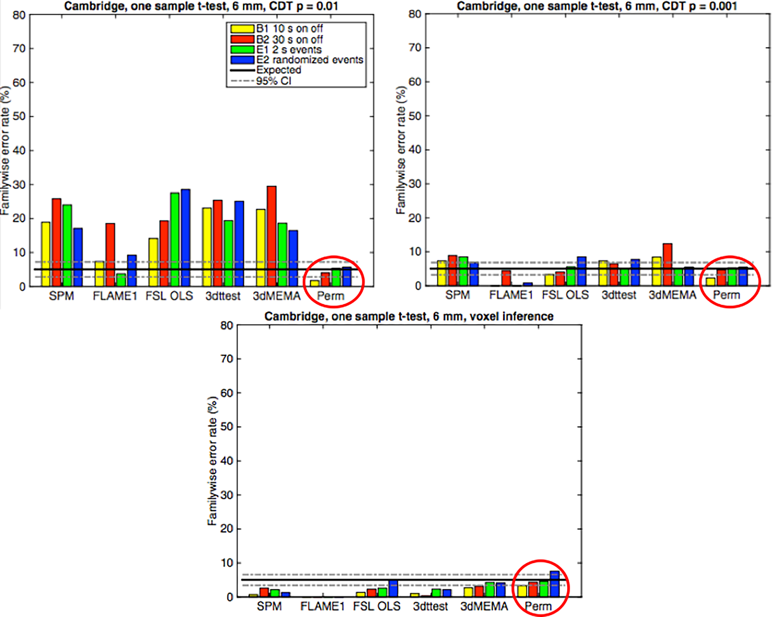
When the authors ran simulations on large datasets under different experimental conditions (e.g., block design and event-related), they found that this assumption of a Gaussian shape led to false positives far above the expected 5% rate across all the major software packages (SPM, AFNI, and FSL). The commonly used p = 0.01 threshold for the individual voxels of the cluster led to much higher false positive rates than a more stringent p = 0.001 threshold. (Notably, permutation testing, a nonparametric method that does not rely on assumptions of normality, did not show any substantial difference in false positives under any conditions.) These inflated false positive rates led to the following figure, which was picked up by the popular media and discussed in a fair, evenhanded way which emphasized that although false positive rates could be increased in some cases, it would be hasty to conclude that all neuroimaging results are wrong.*


Figure 1 from Eklund et al (2016). Simulations on an open-access dataset for different block and event-related designs. Upper left: Cluster-defining threshold (CDT) of p = 0.01 uncorrected; upper right: CDT of p = 0.001 uncorrected; bottom: voxel-level inference. Black line: Expected false positive rate of 5%. A threshold of p = 0.01 leads to inflated false positives across all of the major software packages (SPM, AFNI, and FSL), while a threshold of p = 0.001 leads to clusters closer to the expected 5% false positive rate. Voxel-level inference is slightly conservative in all cases. Permutation testing (circled in red), a nonparametric method, does as expected under all conditions.

*Or not.

Solutions

There are three solutions to this problem; solutions to make neuroimaging respectable again, to cease being laughed at as cranks, charlatans, raiders of the public fisc, and attention-seeking, unscrupulous bloggers.

One solution is to use voxel-wise thresholds; although, as shown in the Eklund paper, these are often far too conservative, and can lead one to conclude there are no results when they actually do exist. I, for one, cannot stand the thought of those poor results slowly suffocating in their little gray coffins, alive but unable to signal for help. With voxel-wise thresholds we stop up our ears with wax; we think we hear the dim scratching of nails, the whimpers for succor, but dismiss them as figments of a fevered imagination; and we leave those tiny blobs and their tiny blob families to know that their last moments will be horror.

The second, more humane solution is to use more conservative cluster-forming thresholds, such as p = 0.001 uncorrected, in conjunction with more accurate modeling of the spatial autocorrelation. I recommend updating your AFNI binaries to the latest version (i.e., the beginning of 2017 or later), and using the  -acf option in 3dFWHMx. For example:

3dFWHMx -mask mask+tlrc.HEAD -acf tmp.txt errts+tlrc.HEAD

Which will generate parameters for a more accurate estimation of the empirical ACF; you will see something like this:

++start ACF calculations out to radius = 37.68mm
+ACF done (0.74 CPU s thus far)
11.8132 13.748 12.207 12.5629
0.260939 6.36019 16.6387 19.1419 

The first line of numbers are the traditional smoothness estimates in the x-, y-, and z-directions, as well as a weighted average of them (bolded). The second line of numbers are the a, b, and c parameters for the ACF model,

a^(-r*r/(2*b*b))+(1-a)^(-r/c)

With the last number being an updated estimate of the smoothness. These are then input into 3dClustSim:

3dClustSim -acf 0.26 6.36 16.64 -mask mask+tlrc.HEAD -athr 0.05 -pthr 0.001

The difference between the two smoothness estimates leads to substantial differences in significant cluster thresholds. In this case, the traditional estimates lead to a cluster threshold of 668 contiguous voxels, while the ACF version gives a threshold of 1513. This was using an initial cluster-defining threshold of p = 0.01, which can lead to such large differences; more stringent thresholds (e.g., p = 0.001) have less of a difference, but still a significant gap between them.

The third solution is to use non-parametric methods, such as permutation tests; which, since they do not rely on assumptions of normality, are immune to the autocorrelation assumptions listed above. Some popular tools include SPM's SnPM (Statistical non-Parametric Mapping); FSL's randomise; and Eklund's BROCCOLI. Out of the three, I've only used randomise, and found it straightforward to use (see the tutorial here).


Conclusions

Have we been profiting too long from dubious methods in neuroimaging? Have we become lax and complacent in our position as a period science, knowing that no matter how poorly designed the experiment is, no matter how ludicrous the question we are investigating - such as where the word YOLO is in the brain, or how the consumption of Four Loko affects delayed discounting - no matter whether our subjects are technically alive or not, we will probably still get a significant result, most likely in the precuneus?**

The answer to all of these, I would say, is yes. But just because I was able to get the results of my first paper to squeak by with an outdated version of AlphaSim, and consequently have an easy time in graduate school, make tons of money, and be envied by all of my friends, doesn't mean that you should have the same privilege. The way forward will be a hard one for the neuroimagers of today; standards will be higher, methods tighter, reviews harsher. But if you put in enough work, if you exercise enough diligence, and if you live long enough into the ninth year of your graduate program, you may just be able to take advantage of the next major statistical loophole that comes along. Have faith.***


**For the record, I still don't know where the precuneus is. My best guess is: "Somewhere right before the cuneus."

***In all seriousness, AFNI has been responsive, helpful, and, given the circumstances, even gracious with any issues that have come up with their programs - specifically, 3dFWHMx (the smoothness estimator) and 3dClustSim (the cluster threshold estimator). The problems are not so much with AFNI, as with how it is used; and even though it is being patched, it is worth keeping in mind that there will likely be other issues discovered in the future, as with all methods - even non-parametric ones. (Their response to the Eklund paper can be found here.) The responsibility of the user is to make sure that the results that are reported follow the most up-to-date correction methods; that suspicious-looking activations that don't make sense in the experimental context, or consist of several blobs connected by threads of voxels, should be interpreted with caveats; and that even results which are weak and do not pass correction with the current methods, may still be real but underpowered effects. As with any result, it's up to the researcher to use their best judgment.

Friday, July 29, 2016

fMRI Power Analysis with NeuroPower


One of my biggest peeves is complaints about how power analyses are too hard. I often hear things like "I don't have the time," or "I don't know how to use Matlab," or "I'm being held captive in the MRI control room by a deranged physicist who thinks he is taking orders from the Quench button."

Well, Mr. Whiny-Pants, it's time to stop making excuses - a new tool called NeuroPower lets you do power analyses quickly and easily, right from your web browser. The steps are simple: Upload a result from your pilot study, enter a few parameters - sample size, correction threshold, credit card number - and, if you listen closely, you can hear the electricity of the Internet go booyakasha as it finishes your power analysis. Also, if a few days later you notice some odd charges on your credit card statement, I know nothing about that.

The following video will help you use NeuroPower and will answer all of your questions about power analysis, including:

  • What is a power analysis?
  • Why should I do a power analysis?
  • Why shouldn't I do a power analysis on a full dataset I already collected?
  • How much money did you spend at Home Depot to set up the lighting for your videos?
  • What's up with the ducks? "Quack cocaine"? Seriously?

All this, and more, now in 1080p. Click the full screen button for the full report.


Thursday, January 7, 2016

Mumford & Stats: Up Your Neuroscience Game


Jeanette Mumford, furious at the lack of accessible tutorials on neuroimaging statistics, has created her own Tumblr to distribute her knowledge to the masses.

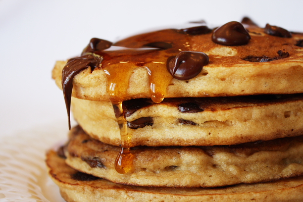
I find examples like these heartening; researchers and statisticians providing help to newcomers and veterans of all stripes. Listservs, while useful, often suffer from poorly worded questions, opaque responses, and overspecificity - the issues are individual, and so are the answers, which go together like highly specific shapes of toast in a specialized toaster.* Tutorials like Mumford's are more like pancake batter spread out over a griddle, covering a wide area and seeping into the drip pans of understanding, while being sprinkled with chocolate chips of insight, lightly buttered with good humor, and drizzled with the maple syrup of kindness.

I also find tutorials like these useful because - let's admit it - we're all slightly stupid when it comes to statistics. Have you ever tried explaining it to your dad, and ended up feeling like a fool? Clearly, we need all the help we can get. If you've ever had to doublecheck why, for example, a t-test works the way it does, or brush up on how contrast weights are made, this website is for you. (People who never had to suffer to understand statistics, on the other hand, just like people who don't have any problems writing, are disgusting and should be avoided.)

Jeanette has thirty-two videos covering the basics of statistics and their application to neuroimaging data, a compression of one of her semester-long fMRI data courses which should be required viewing for any neophyte. More recent postings report on developments and concerns in neuroimaging methods, such as collinearity, orthogonalization, nonparametric thresholding, and whether you should date fellow graduate students in your cohort. (I actually haven't read all of the posts that closely, but I'm assuming that something that important is probably in there somewhere.) And, unlike myself, she doesn't make false promises and she posts regularly; you get to stay current on what's hot, what's not, and, possibly, you can begin to make sense of those knotty methods sections. At least you'll begin to make some sense of the gibberish your advisor mutters in your general direction the next time he wants you to do a new analysis on the default pancake network - the network of regions that is activated in response to a contrast of pancakes versus waffles, since they are matched on everything but texture.**

It is efforts such as this that make the universe of neuroimaging, if not less complex, at least more comprehensible, less bewildering; more approachable, less terrifying. And any effort like that deserves its due measure of praise and pancakes.


*It was only after writing this that I realized you put bread into a toaster - toast is what comes out - but I decided to just own it.

**Do not steal this study idea from me.

Tuesday, May 26, 2015

K-Means Analysis with FMRI Data

Clustering, or finding subgroups of data, is an important technique in biostatistics, sociology, neuroscience, and dowsing, allowing one to condense what would be a series of complex interaction terms into a straightforward visualization of which observations tend to cluster together. The following graph, taken from the online Introduction to Statistical Learning in R (ISLR), shows this in a two-dimensional space with a random scattering of observations:


Different colors denote different groups, and the number of groups can be decided by the researcher before performing the k-means clustering algorithm. To visualize how these groups are being formed, imagine an "X" being drawn in the center of mass of each cluster; also known as a centroid, this can be thought of as exerting a gravitational pull on nearby data points - those closer to that centroid will "belong" to that cluster, while other data points will be classified as belonging to the other clusters they are closer to.

This can be applied to FMRI data, where several different columns of data extracted from an ROI, representing different regressors, can be assigned to different categories. If, for example, we are looking for only two distinct clusters and we have several different regressors, then a voxel showing high values for half of the regressors but low values for the other regressors may be assigned to cluster 1, while a voxel showing the opposite pattern would be assigned to cluster 2. The label itself is arbitrary, and is interpreted by the researcher.

To do this in Matlab, all you need is a matrix with data values from your regressors extracted from an ROI (or the whole brain, if you want to expand your search). This is then fed into the kmeans function, which takes as arguments the matrix and the number of clusters you wish to partition it into; for example, kmeans(your_matrix, 3).

This will return a vector of numbers classifying a particular row (i.e., a voxel) as belonging to one of the specified clusters. This vector can then be prefixed to a matrix of the x-, y-, and z-coordinates of your search space, and then written into an image for visualizing the results.

There are a couple of scripts to help out with this: One, createBlankNIFTI.m, which will erase a standardized space image (I suggest a mask output by SPM at its second level) and replace every voxel with zeros, and the other script, createNIFTI.m, will fill in those voxels with your cluster numbers. You should see something like the following (here, I am visualizing it in the AFNI viewer, since it automatically colors in different numbers):

Sample k-means analysis with k=3 clusters.

The functions are pasted below, as well as a couple of explanatory videos.


function createBlankNIFTI(imageFile)

%Note: Make sure that the image is a copy, and retain the original

X = spm_read_vols(spm_vol(imageFile));
X(:,:,:) = 0;
spm_write_vol(spm_vol(imageFile), X);


=================================

function createNIFTI(imageFile, textFile)


hdr = spm_vol(imageFile);
img = spm_read_vols(hdr);

fid = fopen(textFile);
nrows = numel(cell2mat(textscan(fid,'%1c%*[^\n]')));
fclose(fid);

fid = 0;


for i = 1:nrows
    if fid == 0
        fid = fopen(textFile);
    end
    
    Z = fscanf(fid, '%g', 4);
    
    img(Z(2), Z(3), Z(4)) = Z(1);
    spm_write_vol(hdr, img);
end


Saturday, May 9, 2015

Leave One Subject Out Cross Validation - The Video

Due to the extraordinary popularity of the leave-one-subject-out (LOSO) post I wrote a couple of years ago, and seeing as how I've been using it lately and want to remember how to do it, here is a short eight-minute video on how to do it in SPM. While the method itself is straightforward enough to follow - GLMs are estimated for each group of subjects excluding one subject, and then estimates are extracted from the resulting ROIs for just that subject - the major difficulty is batching it, especially if there are many subjects.

Unfortunately I haven't been able to figure this out satisfactorily; the only advice I can give is that once you have a script that can run your second-level analysis, loop over it while leaving out consecutive subjects for each GLM. This will leave you with the same number of second-level GLMs as there are subjects, and each of these can be used to load up contrasts and observe the resulting clusters from that analysis. Then you extract data from your ROIs for that subject which was left out for the GLM and build up a vector of datapoints for each subject from each GLM, and do t-tests on it, put chocolate sauce on it, eat it, whatever you want. Seriously. Don't tell me I'm the only one who's thought of this.

Once you have your second-level GLM for each subject, I recommend using the following set of commands to get that subject's unbiased data (I feel slightly ridiculous just writing that: "unbiased data"; as though the data gives a rip about anything one way or the other, aside from maybe wanting to be left alone, and just hang out with its friends):

1. Load up your contrast, selecting your uncorrected p-value and cluster size;
2. Click on your ROI and highlight the corresponding coordinates in the Results windown;
3. Find out what the path is to the contrasts for each subject for that second-level contrast by typing "SPM.xY.P"; that will be the template you will alter to get the single subject's data - for example, "/data/myStudy/subject_101/con_0001.img" - and then you can save this to a variable, such as "subject_101_contrast";
4. Average that subject's data across the unbiased ROI (there it is again! I can't get away from it) using something like "mean(spm_get_data(subject_101_contrast, xSPM.XYZ), 2)";
5. Save the resulting value to a vector, and update this for each additional subject.


Friday, April 17, 2015

Slice Analysis of FMRI Data with SPM


Slice analysis is a simple procedure - first you take a jar of peanut butter and a jar of Nutella, and then use a spoon to take some Nutella and then use the same spoon to mix it with the peanut butter. Eat and repeat until you go into insulin shock, and then...

No, wait! I was describing my midnight snack. The actual slice analysis method, although less delicious, is infinitely more helpful in determining regional dissociations of activity, as well as avoiding diabetes. (Although who says they can't both be done at the same time?)

The first step is to extract contrast estimates for each slice from a region of interest (ROI, also pronounced "ROY") and then average across all the voxels in that slice for the subject. Of course, there is no way you would be able to do this step on your own, so we need to copy someone else's code from the Internet and adapt it to our needs; one of John Ashburner's code snippets (#23, found here) is a good template to start with. Here is my adaptation:


rootdir = '/data/drill/space10/PainStudy/fmri/'; %Change these to reflect your directory structure
glmdir = '/RESULTS/model_RTreg/'; %Path to SPM.mat and mask files

subjects = [202:209 211:215 217 219 220:222 224:227 229 230 232 233];
%subjects = 202:203;

Conditions.names = {'stroopSurpriseConStats', 'painSurpriseConStats'}; %Replace with your own conditions
Masks = {'stroopSurpriseMask.img', 'painSurpriseMask.img'}; %Replace with your own masks; should be the product of a binary ROI multiplied by your contrast of interest
Conditions.Contrasts = {'', ''};

ConStats = [];
Condition1 = [];
Condition2 = [];

for i=subjects
    
    cd([rootdir num2str(i) glmdir])
    outputPath = [rootdir num2str(i) glmdir]; %Should contain both SPM.mat file and mask files
    
    for maskIdx = 1:length(Masks)
      
    P = [outputPath Masks{(maskIdx)}];

    V=spm_vol(P);

    tmp2 = [];
    
     [x,y,z] = ndgrid(1:V.dim(1),1:V.dim(2),0);
     for i=1:V.dim(3),
       z   = z + 1;
       tmp = spm_sample_vol(V,x,y,z,0);
       msk = find(tmp~=0 & isfinite(tmp));
       if ~isempty(msk),
         tmp = tmp(msk);
         xyz1=[x(msk)'; y(msk)'; z(msk)'; ones(1,length(msk))];
         xyzt=V.mat(1:3,:)*xyz1;
         for j=1:length(tmp),
           tmp2 = [tmp2; xyzt(1,j), xyzt(2,j), xyzt(3,j), tmp(j)];
         end;
       end;
     end;

         xyzStats = sortrows(tmp2,2); %Sort relative to second column (Y column); 1 = X, 3 = Z
         minY = min(xyzStats(:,2));
         maxY = max(xyzStats(:,2));

         ConStats = [];

     for idx = minY:2:maxY
         x = find(xyzStats(:,2)==idx); %Go in increments of 2, since most images are warped to this dimension; however, change if resolution is different
         ConStats = [ConStats; mean(xyzStats(min(x):max(x),4))];
     end

    if maskIdx == 1
        Condition1 = [ConStats Condition1];
    elseif maskIdx == 2
        Condition2 = [ConStats Condition2];
    end

    end
end

Conditions.Contrasts{1} = Condition1;
Conditions.Contrasts{2} = Condition2;


This script assumes that there are only two conditions; more can be added, but care should be taken to reflect this, especially with the if/else statement near the end of the script. I could refine it to work with any amount of conditions, but that would require effort and talent.

Once these contrasts are loaded into your structure, you can then put them in an Excel spreadsheet or any other program that will allow you to format and save the contrasts in a tab-delimited text format. The goal is to prepare them for analysis in R, where you can test for main effects and interactions across the ROI for your contrasts. In Excel, I like to format it in the following four-column format:


Subject Condition Position  Contrast
202 Stroop 0 -0.791985669
202 Stroop 2 -0.558366941
202 Stroop 4 -0.338829942
202 Pain 0 0.17158524
202 Pain 2 0.267789503
202 Pain 4 0.192473782
203 Stroop 0 0.596162455
203 Stroop 2 0.44917655
203 Stroop 4 0.410870348
203 Pain 0 0.722974284
203 Pain 2 0.871030304
203 Pain 4 1.045700207


And so on, depending on how many subjects, conditions, and slices you have. (Note here that I have position in millimeters from the origin in the y-direction; this will depend on your standardized space resolution, which in this case is 2mm per slice.)

Once you export that to a tab-delimited text file, you can then read it into R and analyze it with code like the following:

setwd("~/Desktop")
x = read.table("SliceAnalysis.txt", header=TRUE)
x$Subject <- as.factor="" font="" ubject="" x="">
aov.x = aov(Contrast~(Condition*Position)+Error(Subject/(Condition*Position)),x)
summary(aov.x)
interaction.plot(x$Position, x$Condition, x$Contrast)


This will output statistics for main effects and interactions, as well as plotting the contrasts against each other as a function of position.

That's it! Enjoy your slices, crack open some jars of sugary products, and have some wild times!


Friday, August 8, 2014

Parametric Modulation with SPM: Why Order Matters

Those who are the youngest children in the family are keenly aware of the disadvantages of being last in the pecking order; the quality of toys, clothes, and nutrition is often best for the eldest children in the family, and gradually tapers off as you reach the last kids, who are usually left with what are called, in parent euphemisms, "hand-me-downs."

In reality, these are things that should have been discarded several years ago due to being broken, unsafe, containing asbestos, or clearly being overused, such as pairs of underwear that have several holes in them so large that you're unsure of where exactly your legs go.

In SPM land, a similar thing happens to parametric modulators, with later modulators getting the dregs of the variance not wanted by the first modulators. Think of variance as toys and cake, and parametric modulators as children; everybody wants the most variance, but only the first modulators get the lion's share of it; the last modulators get whatever wasn't given to the first modulators.

The reason this happens is because when GLMs are set up, SPM uses a command, spm_orth, to orthogonalize the modulators. The first modulator is essentially untouched, but all other modulators coming after it are orthogonalized with respect to the first; and this proceeds in a stepwise function, with the second modulator getting whatever was unassigned to the first, the third getting whatever was unassigned to the second, and so on.

(You can see this for yourself by doing a couple of quick simulations in Matlab. Type x1=rand(10,1), and x2=rand(10,1), and then combine the two into a matrix with xMat = [x1 x2]. Type spm_orth(xMat), and notice that the first column is unchanged, while the second is greatly altered. You can then flip it around by creating another matrix, xMatRev = [x2 x1], and using spm_orth again to see what effect this change has.)

Be aware of this, as this can dramatically alter your results depending on how your modulators were ordered. (If they were completely orthogonal by design, then the spm_orth command should have virtually no impact; but this scenario is rare.) This came to my attention when looking at a contrast of a parametric modulator, which was one of three assigned to a main regressor. In one GLM, the modulator was last, and correspondingly explained almost no variance in the data; while in another GLM, the modulator was first, and loaded on much more of the brain. The following two figures show the difference, using exactly the same contrast and correction threshold, but simply reversing the order of the modulators:


Results window when parametric modulator was the last one in order.


Results window when parametric modulator was the first one in order.

This can be dealt with in a couple of ways:
  1. Comment out the spm_orth call in two scripts used in setting up the GLM: line 229 in spm_get_ons.m, and lines 285-287 in spm_fMRI_design.m. However, this might affect people who actually do want the orthogonalization on, and also this increases the probability that you will screw something up. Also note that doing this means that the modulators will not get de-meaned when entered into the GLM.
  2. Create your own modulators by de-meaning the regressor, inserting your value at the TR where the modulator occurred, then convolving this with an HRF (usually the one in SPM.xBF.bf). If needed, downsample the output to match the original TR.

It is well to be aware of all this, not only for your own contrasts, but to see how this is done in other papers. I recall reading one a long time ago - I can't remember the name - where several different models were used, in particular different models where the modulators were entered in different orders. Not surprisingly, the results were vastly different, although why this was the case wasn't clearly explained. Just something to keep in mind, as both a reader and a reviewer.

I should also point out that this orthogonalization does not occur in AFNI; the order of modulators has no influence on how they are estimated. A couple of simulations should help illustrate this:

Design matrices from AFNI with simulated data (one regressor, two parametric modulators.) Left: PM1 entered first, PM2 second. Right: Order reversed. The values are the same in both windows, just transposed to illustrate which one was first in the model.

More information on the topic can be found here, and detailed instructions on how to construct your own modulators can be found on Tor Wager's lab website.

Friday, August 1, 2014

Blistering Fast Functional Connectivity Analysis with 3dTproject

Because speed is associated with freedom, happiness, and the American way - we want results, we want visible results, and we want them now, darn it! - it is no surprise that neuroimaging analysis is becoming exponentially faster and more efficient. Gone are the days when you could run a slice-timing step, go to bed, and wake up eight hours later when it finally finished. Most likely it crashed, meaning you had to run the entire thing all over again, but that didn't matter - the point was that you at least felt as though you were doing something during that time.

Regardless, we are approaching a radically different era now; and one of the harbingers of that era is AFNI's 3dTproject. Released a few months ago, this tool is now the default in both uber_subject.py and afni_proc.py when you do resting state analyses. It's quicker, more efficient, and allows fewer chances to mess things up, which is a good thing.

To include 3dTproject in your analysis pipeline, simply apply "rest" to the analysis initialization screen when running uber_subject.py, or copy example #9 from the help documentation of afni_proc.py. Under no circumstances should you try running 3dTproject manually, since you, possessing the hand-eye coordination of a cheese burrito, will inevitably make a typo and screw something up. Nevertheless, if you insist on doing it yourself, I recommend using the following code that is automatically generated by the .py scripts:

3dTproject -polort 0 -input pb04.$subj.r*.blur+tlrc.HEAD -censor motion_${subj}_censor.1D -cenmode ZERO -ort X.nocensor.xmat.1D -prefix errts.${subj}.tproject

Needless to say, you will have to have already run your preprocessing steps and have run 3dDeconvolve with the -x1D_stop option to generate the necessary matrices.


Monday, June 23, 2014

Multiple Regression in SPM

A couple of videos have been posted about multiple regression in SPM, both at the first level and second level. Technically, almost all of the GLMs researchers usually set up use multiple linear regression, where a linear combination of weighted regressors is fit to the timecourse of each voxel. However, in SPM parlance, regressors are distinct from conditions: Conditions are typically convolved with some sort of basis function (usually a hemodynamic response function), whereas regressors are not convolved with anything. For example, someone may enter motion parameters as regressors, since they are not convolved with any hemodynamic shape, but still may account for some of the variance observed in the signal (and, we hope, the signal that is primarily due to motion). Another example would be entering in the timecourse extracted from an ROI to do a functional connectivity analysis, or inserting the interaction term from a PPI analysis as a regressor.

At the second level SPM also gives the option for doing multiple regression; but this is simply the entering of covariates which can be tested for correlations with the signal change in contrasts across subjects. In most cases, however, you can select any other design, and enter in covariates regardless of which design that you choose; which I believe to be the better option, since it is more flexible.

In any case, most of the rest of the details can be found in the following videos. Speak hands for me.


Monday, June 16, 2014

Running SPM First-Level Analyses from the Command Line

For most people, doing first-level analyses in SPM is tedious in the extreme; for other people, these analyses are manageable through command line scripting in Matlab. And there are still other people who don't even think about first-level analyses or SPM or Matlab or any of that. This last class of people are your college classmates who majored in something else, like economics, and are living significantly less stressful lives than you, making scads of money, and regularly eating out at restaurants where they serve shrimp the size of Mike Tyson's forearm.

Assuming that you belong to the first category, however, first-level analyses are invariably a crashing bore; and, worse, completely impractical for something like beta-series analysis, where a separate regressor is needed for individual events.

The following script will do all of that for you, although it makes many assumptions about your timing files and where everything is stored. First, your directory needs to be set up with a root directory containing all of the subjects, as well as a separate timing directory containing your onsets files; and second, that the timing files are written in a four-column format of runs, regressors, onsets (in seconds), and duration. Once you have all of that, though, all it takes is simply modifications of the script to run your analysis.

As always, let me know if this actually helps, or whether there are sections of code that can be cleaned up. I will be making a modification tomorrow allowing for beta series analysis by converting all of the timing events into individual regressors, which should help things out.

Link to script: http://mypage.iu.edu/~ajahn/docs/Run_SPM_FirstLevel.m

% INPUT:
%  rootDir        - Path to where subjects are located
%  subjects       - Vector containing list of subjects (can concatenate with brackets)
%  spmDir         - Path to folder where you want to move the multiple conditions .mat files and where to the output SPM file (directory is created if it doesn't
%  exist)
%  timingDir      - Path to timing directory, relative to rootDir
%  timingSuffix   - Suffix appended to timing files
%  matPrefix      - Will be prefixed to output .mat files.
%  dataDir        - Directory storing functional runs.
%
% OUTPUT:
%  One multiple condition .mat file per run. Also specifies the GLM and runs
%  beta estimation.
%       
%
%       Note that this script assumes that your timing files are organized
%       with columns in the following order: Run, ConditionName, Onset (in
%       seconds), Duration (in seconds)
%
%       Ideally, this timing file should be written out from your
%       presentation software, e.g., E-Prime
%
%       Also note how the directory tree is structured in the following example. You may have to
%       change this script to reflect your directory structure.
%       
%       Assume that:
%         rootdir = '/server/studyDirectory/'
%         spmDir = '/modelOutput/'
%         timingDir = '/timings/onsets/'
%         subjects = [101]
%         timingSuffix = '_timing.txt'
%       1) Sample path to SPM directory:
%       '/server/studyDirectory/101/modelOutput/'
%       2) Sample path to timing file in the timing directory:
%       '/server/studyDirectory/timings/onsets/101_timing.txt'
%
% Andrew Jahn, Indiana University, June 2014
% andysbrainblog.blogspot.com

clear all

%%%----Things you will want to change for your study----%%%

rootDir = '/data/hammer/space5/ImagineMove/fmri/';
subjects = [214 215];
spmDir = '/RESULTS/testMultis/';
timingDir = 'fMRI_behav/matlab_input/';
timingSuffix = '_spm_mixed.txt';
matPrefix = 'testMulti';
dataDir = '/RESULTS/data/';

%Change these parameters to reflect study-specific information about number
%of scans and discarded acquisitions (disacqs) per run
funcs = {'swuadf0006.nii', 'swuadf0007.nii', 'swuadf0008.nii'}; %You can add more functional runs; just remember to separate them with a comma
numScans = [240 240 240]; %This if the number of scans that you acquire per run
disacqs = 2; %This is the number of scans you later discard during preprocessing
numScans = numScans-disacqs;
TR = 2; %Repetition time, in seconds

%Estimating the GLM can take some time, particularly if you have a lot of betas. If you just want to specify your
%design matrix so that you can assess it for singularities, turn this to 0.
%If you wish to do it later, estimating the GLM through the GUI is very
%quick.
ESTIMATE_GLM = 1;


%%%-----------------------------------------------------%%%


%For each subject, create timing files and jobs structure
for subject = subjects
    
    %See whether output directory exists; if it doesn't, create it
    outputDir = [rootDir num2str(subject) spmDir];
    
    if ~exist(outputDir)
        mkdir(outputDir)
    end
     
    %---Navigate to timing directory and create .mat files for each run---%
    cd([rootDir timingDir]);
    
    fid = fopen([num2str(subject) timingSuffix], 'rt');
    T = textscan(fid, '%f %s %f %f', 'HeaderLines', 1); %Columns should be 1)Run, 2)Regressor Name, 3) Onset Time (in seconds, relative to start of each run), and 4)Duration, in seconds
    fclose(fid);
    
    clear runs nameList names onsets durations sizeOnsets %Remove these variables if left over from previous analysis
    
    runs = unique(T{1});

    %Begin creating jobs structure
    jobs{1}.stats{1}.fmri_spec.dir = cellstr(outputDir);
    jobs{1}.stats{1}.fmri_spec.timing.units = 'secs';
    jobs{1}.stats{1}.fmri_spec.timing.RT = TR;
    jobs{1}.stats{1}.fmri_spec.timing.fmri_t = 16;
    jobs{1}.stats{1}.fmri_spec.timing.fmri_t0 = 1;

    %Create multiple conditions .mat file for each run
    for runIdx = 1:size(runs, 1)
            nameList = unique(T{2});
            names = nameList';
            onsets = cell(1, size(nameList,1));
            durations = cell(1, size(nameList,1));
            sizeOnsets = size(T{3}, 1);
        for nameIdx = 1:size(nameList,1)
            for idx = 1:sizeOnsets
                if isequal(T{2}{idx}, nameList{nameIdx}) && T{1}(idx) == runIdx
                    onsets{nameIdx} = double([onsets{nameIdx} T{3}(idx)]);
                    durations{nameIdx} = double([durations{nameIdx} T{4}(idx)]);
                end
            end
            onsets{nameIdx} = (onsets{nameIdx} - (TR*disacqs)); %Adjust timing for discarded acquisitions
        end

        save ([matPrefix '_' num2str(subject) '_' num2str(runIdx)], 'names', 'onsets', 'durations')
        
        %Grab frames for each run using spm_select, and fill in session
        %information within jobs structure
        files = spm_select('ExtFPList', [rootDir num2str(subject) dataDir], ['^' funcs{runIdx}], 1:numScans);

        jobs{1}.stats{1}.fmri_spec.sess(runIdx).scans = cellstr(files);
        jobs{1}.stats{1}.fmri_spec.sess(runIdx).cond = struct('name', {}, 'onset', {}, 'duration', {}, 'tmod', {}, 'pmod', {});
        jobs{1}.stats{1}.fmri_spec.sess(runIdx).multi = cellstr([outputDir matPrefix '_' num2str(subject) '_' num2str(runIdx) '.mat']);
        jobs{1}.stats{1}.fmri_spec.sess(runIdx).regress = struct('name', {}, 'val', {});
        jobs{1}.stats{1}.fmri_spec.sess(runIdx).multi_reg = {''};
        jobs{1}.stats{1}.fmri_spec.sess(runIdx).hpf = 128;
        
                
    end
    
    movefile([matPrefix '_' num2str(subject) '_*.mat'], outputDir)
    
    %Fill in the rest of the jobs fields
    jobs{1}.stats{1}.fmri_spec.fact = struct('name', {}, 'levels', {});
    jobs{1}.stats{1}.fmri_spec.bases.hrf = struct('derivs', [0 0]);
    jobs{1}.stats{1}.fmri_spec.volt = 1;
    jobs{1}.stats{1}.fmri_spec.global = 'None';
    jobs{1}.stats{1}.fmri_spec.mask = {''};
    jobs{1}.stats{1}.fmri_spec.cvi = 'AR(1)';
    
    %Navigate to output directory, specify and estimate GLM
    cd(outputDir);
    spm_jobman('run', jobs)
    
    if ESTIMATE_GLM == 1
        load SPM;
        spm_spm(SPM);
    end
    
end

%Uncomment the following line if you want to debug
%keyboard


Sunday, June 15, 2014

Writing Out Timing Files from E-Prime

Now, I promised you all something that would help make running SPM analyses easier; for although we would all like something that is both transparent and usable, in most FMRI packages they are polar of each other. SPM in many ways is very usable; but this tends to be more hindrance than asset when running large groups of subjects, when manually selecting each session and copying and pasting by hand become not only tedious, but dangerous, as the probability of human error is compounded with each step. Best to let the machines do the work for you when you can. Anything else is an affront to them; you'll wake more than just the dogs.

Do assist our future overlords in their work, command lines for each step should be used whenever possible. But, rummily enough, SPM offers little documentation about this, and it more or less needs to be puzzled out on your own. For most processing this wouldn't be too much of a hassle, but there is one step where it is indispensable, more indispensable, if possible, than Nutella on a banana sprinkled with chopped walnuts. Or possibly warm Nutella drizzled on top of vanilla ice cream and left standing until it cools and hardens into a shell. Has anyone tried this? Could you let me know how it tastes? Thanks!

Where was I? Right; the one step where you need batching is first-level analysis, where timing information is entered for each session (or run) for each subject. Back in the autumn of aught eight during my days as a lab technician I used to be just like you, arriving to work in the morning and easing my falstaffian bulk into my chair before starting my mind-numbing task of copying and pasting onset times into each condition for each run, invariably tiring of it after a few minutes but keeping at it, and maybe completing a few subjects by the end of the day. Not the most exciting or fulfilling work, and I probably screwed a lot of things up without noticing it.

SPM has tried to anticipate problems like this by specifying a Multiple Condition option through their interface, where you supply a .mat file for each session that contains all of the names, onsets, and durations for that session, and everything is automatically filled in for you. Which sounds great, until you realize that creating Matlab files is, like, hard, and then you go back to your old routine. (The manual also says that these .mat files can be generated automatically by presentation software such as COGENT, but I have never met anyone who has ever used COGENT; this is, in all likelihood, a fatcat move by Big Science to get you to buy a piece of software that you don't need.)

What we will be doing, then, is trying to make this as straightforward and simple of a process as possible. However, this assumes that you have your onsets organized in a certain way; and first we will talk about how to create those onsets from your stimulus presentation program. This will allow you much more flexibility, as you can choose what you want to write into a simple text file without having to go through copying and pasting data from the E-Prime DataAid program into Excel for further processing.  (I use E-Prime, and will be reviewing that here, but I believe that most presentation programs will allow you to write out data on the fly.)

Within E-Prime, you will need to know exactly when the scanner started, and use this as time zero for your onsets files. I usually do this by having a screen that says "Waiting for scanner..." which only terminates once the scanner sends a trigger pulse through a USB cord hooked up to the presentation laptop. We have a Siemens Trio scanner, which sends a backtick ( ` ); check whether your scanner does the same.


Note that I have an inline script (i.e., an object that contains E-Basic code) right after the WaitScanner slide that contains the following code:

StartTimestamp = CLng(c.GetAttrib("WaitScanner.RTTime")
c.SetAttrib "StartTimestamp", StartTimestamp

if c.GetAttrib("Session") = 1 Then

Open "OnsetTimes_" & c.GetAttrib("Subject") & ".txt" For Output as #1
Close #1

Open "OnsetTimes_" & c.GetAttrib("Subject") & ".txt" For Append As #1
      Print #1, "Run", "Event", "Onset", "Dur"
Close #1

end if


Also, in the duration/input tab for the properties of waitscanner, I have the Keyboard accepting ( ` ) as an input, and termination when it receives that backtick. The StartTimestamp will simply record when the scanner first started, and the if/then statement ensures that the file does not get overwritten when the next run is started.

After that, the StartTimestamp variable and the newly create text file can be used to record information after each event, with the specified condition being determined by you. To calculate the timing for each event, all you have to do is grab the onset time of a condition through the c.GetAttrib command, and subtract the StartTimestamp variable from that:


Additional runs will continue to append to the text file, until you have all of the timing information that you need for your subject. This can then be parsed by a script and divided into multiple condition .mat files, which we will discuss tomorrow.

Thursday, June 12, 2014

Beta Series Analysis in SPM

The following is a script to run beta series analysis in SPM; which, conceptually, is identical to beta series analysis in AFNI, just made more complicated by the use of Matlab commands, many of which I would otherwise remain totally ignorant of.

Also, if you believe that I did this on my own, you are a scoundrel and a fool. Virtually all of the code is from my colleague Derek Nee, a postdoc who used to work in my lab and who remains my superior in all things, scientific and otherwise. He also once got me with the old "If you say gullible slowly, it sounds like orange" joke.

In any case, all that I did was repackage it into a function to be more accessible by people outside of our lab. You may see a couple snippets of code that are useful outside of just doing beta series analysis; for example, the spm_get_data command, which can be used for parameter extraction from the command line without using marsbar. Also note that the script assumes that each trial for a condition has been labeled separately with the regressor name followed by a "_" and then the occurrence of the trial. So, for example, if I were looking at 29 instances of pressing the left button, and the regressor name was LeftButtonPress, I would have LeftButtonPress_1, LeftButtonPress_2, LeftButtonPress_3...LeftButtonPress_29.

Obviously, this is very tedious to do by hand. The Multiple Conditions option through the SPM GUI for setting up 1st level analyses is indispensable; but to cover that is another tutorial, one that will probably cross over into our discussion of GLMs.


The script:

function DoBetaSeries(rootdir, subjects, spmdir, seedroi, Conds, MapNames)
% function BetaSeries(rootdir, subjects, spmdir, seedroi, Conds, MapNames)
% INPUT:
%  rootdir  - Path to where subjects are stored
%  subjects - List of subjects (can concatenate with brackets)
%  spmdir   - Path to folder containing SPM file
%  seedroi  - Absolute path to file containing ROI in NIFTI format
%  Conds    - List of conditions for beta series analysis
%  MapNames - Output for list of maps, one per Conds cell
%       
%   Example use:
%       BetaSeries('/data/study1/fmri/', [101 102 103],
%       'model/BetaSeriesDir/', '/data/study1/Masks/RightM1.nii',
%       {'TapLeft'}, {'TapLeft_RightM1'})
%
%       conditions to be averaged together should be placed together in a cell
%       separate correlation maps will be made for each cell
%       Conds = {'Incongruent' 'Congruent' {'Error' 'Late'}}; 
%
%       For MapNames, there should be one per Conds cell above
%       e.g., with the Conds above, MapNames = {'Incongruent_Map',
%       'Congruent_Map', 'Error_Late_Map'}
%
%       Once you have z-maps, these can be entered into a 2nd-level
%       1-sample t-test, or contrasts can be taken between z-maps and these
%       contrasts can be taken to a 1-sample t-test as well.
%
% 

if nargin < 5
 disp('Need rootdir, subjects, spmdir, seedroi, Conds, MapNames. See "help BetaSeries" for more information.')
    return
end


%Find XYZ coordinates of ROI
Y = spm_read_vols(spm_vol(seedroi),1);
indx = find(Y>0);
[x,y,z] = ind2sub(size(Y),indx);
XYZ = [x y z]';


%Find each occurrence of a trial for a given condition
%These will be stacked together in the Betas array
for i = 1:length(subjects)
    subj = num2str(subjects(i));
    disp(['Loading SPM for subject ' subj]);
    %Can change the following line of code to CD to the directory
    %containing your SPM file, if your directory structure is different
    cd([rootdir subj filesep spmdir]);
    load SPM;
    
    for cond = 1:length(Conds)
        Betas = [];
        currCond = Conds{cond};
        if ~iscell(currCond)
            currCond = {currCond};
        end
        for j = 1:length(SPM.Vbeta) 
            for k = 1:length(currCond)
                if ~isempty(strfind(SPM.Vbeta(j).descrip,[currCond{k} '_'])) 
                    Betas = strvcat(Betas,SPM.Vbeta(j).fname);
                end
            end
        end
              

    %Extract beta series time course from ROI
    %This will be correlated with every other voxel in the brain
    if ischar(Betas)
        P = spm_vol(Betas);
    end

    est = spm_get_data(P,XYZ);
    est = nanmean(est,2);


        %----Do beta series correlation between ROI and rest of brain---%

            MapName = MapNames{cond};
            disp(['Performing beta series correlation for ' MapName]);
            
            Vin = spm_vol(Betas);
            nimgo = size(Vin,1);
            nslices = Vin(1).dim(3);

            % create new header files
            Vout_r = Vin(1);   
            Vout_p = Vin(1);
            [pth,nm,xt] = fileparts(deblank(Vin(1).fname));
            Vout_r.fname = fullfile(pth,[MapNames{cond} '_r.img']);
            Vout_p.fname = fullfile(pth,[MapNames{cond} '_p.img']);

            Vout_r.descrip = ['correlation map'];
            Vout_p.descrip = ['p-value map'];

            Vout_r.dt(1) = 16;
            Vout_p.dt(1) = 16;

            Vout_r = spm_create_vol(Vout_r);
            Vout_p = spm_create_vol(Vout_p);

            % Set up large matrix for holding image info
            % Organization is time by voxels
            slices = zeros([Vin(1).dim(1:2) nimgo]);
            stack = zeros([nimgo Vin(1).dim(1)]);
            out_r = zeros(Vin(1).dim);
            out_p = zeros(Vin(1).dim);


            for i = 1:nslices
                B = spm_matrix([0 0 i]);
                %creates plane x time
                for j = 1:nimgo
                    slices(:,:,j) = spm_slice_vol(Vin(j),B,Vin(1).dim(1:2),1);
                end

                for j = 1:Vin(1).dim(2)
                    stack = reshape(slices(:,j,:),[Vin(1).dim(1) nimgo])';
                    [r p] = corr(stack,est);
                    out_r(:,j,i) = r;
                    out_p(:,j,i) = p;

                end

                Vout_r = spm_write_plane(Vout_r,out_r(:,:,i),i);
                Vout_p = spm_write_plane(Vout_p,out_p(:,:,i),i);

            end

                
            %Convert correlation maps to z-scores
            %NOTE: If uneven number of trials in conditions you are
            %comparing, leave out the "./(1/sqrt(n-3)" term in the zdata
            %variable assignment, as this can bias towards conditions which
            %have more trials
            
                disp(['Converting correlation maps for subject ' subj ', condition ' MapNames{cond} ' to z-scores'])
                P = [MapNames{cond} '_r.img'];
                n = size(Betas,1);
                Q = MapNames{cond};
                Vin = spm_vol([MapNames{cond} '_r.img']);

                % create new header files
                Vout = Vin;   

                [pth,nm,xt] = fileparts(deblank(Vin(1).fname));
                Vout.fname = fullfile(pth,[Q '_z.img']);

                Vout.descrip = ['z map'];

                Vout = spm_create_vol(Vout);

                data = spm_read_vols(Vin);
                zdata = atanh(data)./(1/sqrt(n-3));

                spm_write_vol(Vout,zdata);

    end
end


This can either be copied and pasted into a script, or downloaded as a .m file here.


Friday, June 6, 2014

Independent Components Analysis, Part II: Using FSL Example Data

For our next step, we will be working with FSL example data - somewhat artificial data, true, and much better quality than anything you can ever expect from the likes of your data, which will only lead to toil, sweat, and the garret. Sufficient unto the day is the frustration thereof.

However, it is a necessary step to see what ICA analysis ought to look like, as well as learning how to examine and identify components related to tasks and networks that you are interested in. Also - and possibly more important - you will learn to recognize sources of noise, such as components related to head motion and physiological artifacts.

First, go to the link http://fsl.fmrib.ox.ac.uk/fslcourse/ and scroll to the bottom for instructions on how to download the datasets. You can use either wget or curl. For this demonstration, we will be using datasets 2 and 6:

curl -# -O -C - http://fsl.fmrib.ox.ac.uk/fslcourse/fsl_course_data2.tar.gz
curl -# -O -C - http://fsl.fmrib.ox.ac.uk/fslcourse/fsl_course_data6.tar.gz


Once you have downloaded them, unzip them using gunzip, and then "tar -xf" on the resulting tar files. This will create a folder called fsl_course_data, which you should rename so that they do not conflict with each other. Within fsl_course_data2, navigate to the /melodic/av directory, where you will find a small functional dataset that was acquired while the participant was exposed to auditory stimuli and visual stimuli - which sounds much more scientific than saying, "The participant saw stuff and heard stuff."

Open up the MELODIC gui either through the FSL gui, or through typing Melodic_gui from the command line. Most of the preprocessing steps can be kept as is. However, keep the following points in mind:

1. Double-check the TR. FSL will fill it in automatically from the header of the NIFTI file, but it isn't always reliable.

2. Spatial smoothing isn't required in ICA, but a small amount can help produce better-looking and more identifiable component maps. Somewhere on the order of the size of a voxel or two will usually suffice.


3. By default, MELODIC automatically estimates the number of components for you. However, if you have severe delusions and believe that you know how many components should be generated, you can turn off the "Automatic dimensionality estimation" option in the Stats tab, and enter the number of components you want.


4. The Threshold IC maps option is not the same thing as a p-value correction threshold. I'm not entirely clear on how it relates to the mixture modeling carried out by ICA, but my sense from reading the documentation and papers using ICA is that a higher threshold only keeps those voxels that have a higher probability of belonging to the true signal distribution, instead of the background noise distribution, and it comes down to a balance between false positives and false negatives. I don't have any clear guidelines about what threshold to use, but I've seen cutoffs used within the 0.8-0.9 range in papers.


5. I don't consider myself a snob, but I was using the bathroom at a friend's house recently, and I realized how uncomfortable that cheap, non-quilted toilet paper can be. It's like performing intimate hygiene with roofing materials.


6. Once you have your components, you can load them into FSLview and scroll through them with the "Volumes" button in the lower left corner. You can also load the Atlases from the Tools menu and double-click on it to get a semi-transparent highlight of where different cortical regions are. This can be useful when trying to determine whether certain components fall within network areas that you would expect them to.


More details in the videos below, separately for the visual-auditory and resting-state datasets.