Guidelines for Conducting FMRI Studies: Reliability Issues

Since FMRI data is (mostly) crap - but extremely expensive crap - there is much debate over how experiments should be designed in order to maximize both power and efficiency. My opinion is that most of these issues would be null if we simply precluded doing any experiments which study trivial or useless things. For example, I have in front of me a paper discussing the neural correlates of heterosexual attraction among females, which used a sample of thirty-nine subjects. Assuming that experiment took about an hour and each scanning hour cost about $500, we can guess that this study cost upwards of $20,000. And all this to study a question that has been answered long ago, as common sense and my own observations suggest that females are irresistibly attracted to the soft, slightly pudgy build of the neuroscience blogger.

For those who must conduct such experiments, however, there are guidelines for balancing the tradeoff between efficiency and reliability (or, the probability that an independent study will replicate your results). In a study conducted by Thirion et al (2007), a large sample of 81 subjects was partitioned into different numbers of subgroups: 2 groups of 40 each, 3 groups of 27 each, 4 groups of 20 each, and so on, to test whether there is a noticeable cutoff for reproducible effects below a specific group size. Further parameters were tested, such as group-level variability and and sensitivity of different p-thresholds.

Figure 1 reproduced from Thirion et al (2007). The top two rows in (a) represent activation maps for disjoint groups of subjects from the same sample; (b) is the group-level statistical map. Note the spread in activation profiles between each of the disjoint groups.

The authors found that an optimal number of subjects to balance both reliability and statistical sensitivity (that is, the ability to detect an effect that is actually present) is about N=25-27, with diminishing returns after that. In addition, the authors counsel the use of mixed-effects models, which take into account variance from first-level analyses (i.e., individual subjects), and downweight subjects with high variability. This procedure is similar to the one employed in FSL's FLAME and AFNI's 3dMEMA.

Figure 8 reproduced from Thirion et al (2007). Both Kappa (a measure of reliability) and activated voxels increase significantly up to around 27 subjects, with a plateau shortly after that.

As a side note, besides merely testing for statistical significance (which is virtually guaranteed with a large enough sample), effect sizes should also be calculated to measure the...well, size of your effect. Essentially all an effect size is, is quantifying the magnitude of the difference between your calculated mean and the null hypothesis mean, in terms of standard deviations. The following table will help you qualify how big your effect is when describing the result:

0-0.3: Wee
0.3-0.5: Not so wee
0.5+: Friggin' HUGE


More details, along with a description of why cluster-thresholding is a better methods than whole-brain corrected voxels, can be found in the original paper.

Andy's Brain Blog Brain Food: Mom's Homemade Granola

You can really taste the vitamins

Back in the good old days, when I first started graduate school, I had a hard time coming up with a good snack for those long afternoon stretches between lunch at noon and going home around two-thirty. Fortunately, I recently rediscovered this classic recipe, which is sweet, delicious, nutritious, and packed with enough fiber to keep your hunger at bay for long periods of time.

You may ask, why is it called Mom's Homemade Granola? Maybe because it's my Mom's recipe, and because she makes it at home. If it were called Goathumper Bill's Granola, you would expect it to be made by some crazy guy out on a farm somewhere diddling livestock. Pay attention.


Anyway, the ingredients are:

• 1 cup old-fashioned oats
• 1/4 cup wheat germ (not toasted)
• 1/4 cup sweetened flaked coconut
• 1/4 cup coarsely broken cashews
• 1/4 cup coarsely broken walnuts or pecans
• 3 teaspoons sesame seeds (or sunflower seeds)
• 1/4 cup pure maple syrup
• 2 tablespoons vegetable oil
• 1 tablespoon brown sugar
• 1 tablespoon light molasses
• 1/2 teaspoon ground cinnamon
• 1/4 cup raisins
• 1/4 cup chopped dried apricots

Preheat the oven to 350 degrees, and then mix the first six ingredients in a large bowl. Whisk the maple syrup and next four ingredient in a medium bowl. Add wet ingredients to dry ingredients; stir to coat evenly. Transfer to a large rimmed baking sheet and spread out the mixture in an even layer. Bake for 8 minutes and then stir, bringing the bottom layer to the top. Bake for 8 minutes longer until golden brown, and then mix in the raisins and apricots. Bake until the fruit is heated through and the granola is slightly darker, and cool completely on the sheet.

I tend to put aluminum foil on the baking sheet and then spread the mixture on top of that; that way, it prevents any of the mixture from sticking to the pan, and you can pick up the foil and funnel the entire mixture easily into a container. Lastly, I also like to substitute agave nectar for the syrup; its viscosity is somewhere in between maple syrup and honey, and I think it tastes better after it is baked. In any case, whatever you do, don't tell Goathumper Bill, or his childhood friend, Melvin the Melon Mounter.

Unbiased FMRI Analysis: Leave One Subject Out

Neuroimaging researchers are incessantly bedeviled by the problem of biased region of interest (ROI) analysis. One is constantly lured by the siren song of significant results and large effect sizes radiating from the stygian depths of a non-independent ROI; and while one can at times point toward their use of independent ROIs from other studies, there is always the lurking suspicion that the researcher already knew where the activation was before the ROI was chosen. I have witnessed men, otherwise Samsons in the field and Solomons in counsel, who have had their heads shorn by the harlot of biased analysis.

The most straightforward and appropriate way to do this, of course, is with a region defined on a priori assumptions about where your quarry might lie, based on theory or based on the results of other studies. This ensures that any results extracted from that region are uninfluenced by the model used to generate the statistical maps, therefore circumventing the issue of "double-dipping", or circular analyses (see Kriegeskorte et al, 2009). Another method is to use anatomical regions based on atlases, which again should be motivated by theory.

However, there is yet another option that I was unaware of until recently: Leaving one subject out (LOSO). According to this procedure, non-independence can be mitigated by constructing a general linear model (GLM) with every subject in the study except for one; statistics such as beta weights, time courses, etc., can then be extracted from the resulting parametric map for the subject that was left out, as this subject is no longer contributing to the signal observed in the given region. This process is then repeated and the appropriate parameter extracted for each subject. It is unlikely that there will be perfect overlap between all of the subjects included in each LOSO analysis, but if the effect is real and robust, then it should survive each of these non-overlapping regions.

One consideration with this procedure is what threshold to use for each LOSO analysis. One approach is to hold the p-value constant, in which case a higher t-threshold is used for each analysis due to a reduction in the degrees of freedom. The other approach is to hold the t-value constant, leading to a slightly increased p-value. Both approaches are defensible, although if there are wide variations in the ROI results with each approach, one may want to reconsider the reliability of their finding.

More details can be found in the paper by Esterman et al (2010); I hope this provides the necessary edification and enlightenment for those benighted souls wading about in the filth of their own squalor.

AFNI Command of the Week: cdf

Not necessarily a neuroimaging-specific tool, cdf simply converts between p-values and t-statistics (or F-statistics) using the cumulative distribution function. Supply the test that you did, followed by the t-statistic (or p-value) and degrees of freedom, e.g.:

cdf -t2p fitt 3.4 15
p = 0.00396 #A t-statstic of 3.4 with 15 degrees of freedom yields a p-value of 0.00396

cdf -p2t fitt 0.001 30
t = 3.65 #We would need a t-statistic of 3.65 or greater to reach a p-value of 0.001

Degrees of freedom can be found by using 3dinfo on a statistical dataset, and then looking at the value of "statpar" associated with your statistical test of interest. Degrees of freedom can also be calculated as the number of time points minus the number of regressors in your model; for example, if you have 1200 time points and 40 regressors, then the degrees of freedom will be 1200-40 = 1160. In the following X-matrix (generated by the command "aiv X.jpg"), the first 25 columns represent regressors accounting for any drift during that run; the next nine columns are the regressors of interest; and the last six columns are motion regressors.

 

The degrees of freedom in neuroimaging data can be a little tricky to interpret, as FMRI time series are temporally autocorrelated; in other words, the value of one time point can be predicted, to a degree, by neighboring timepoints. Therefore, using ordinary GLM estimation techniques can lead to an inflated degrees of freedom. To rectify this, instead of using 3dDeconvolve, use 3dREMLfit, which will attempt to account for this autocorrelation.

Central Limit Theorem Part 2: Retaliation

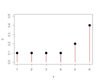
Discrete population, with different probabilities associated with different numbers

Sampling distribution of means from the discrete parent population, with a sample size of n=30

In the last post, we left the central limit theorem defined as a normally-distributed sampling distribution of means reflecting the shape of the normally-distributed parent population, but with a smaller spread and less variance. However, what happens when we sample from a non-normal distribution, such as an exponential distribution or a discrete distribution?

As it turns out, the sampling distribution of means is also normal, regardless of the shape of the parent population. This holds for sample sizes of about 30 or more, which is why the central limit theorem is also sometimes referred to as the law of large numbers.

This is shown in the following video, and can be modified with this R script.

The Central Limit Theorem: Part 1

Random sample of numbers from a normal distribution, N ~ (100, 10). Actual normal distribution is superimposed in red.

One fundamental concept for hypothesis testing is something called the Central Limit Theorem. This theorem states that, for large enough sample sizes and for enough samples, we begin to build a sampling distribution that is approximately normal. More importantly, when we build sampling distributions of the means selected from a population, the average mean is identical to the mean of the parent population.

To illustrate this in R, from the parent population we can take random samples of several different sizes - 10, 50, 300 - and plot those samples as a histogram. These samples will roughly follow the shape of the population they were drawn from - in this case, the normal distribution with a mean of 100 and a standard deviation of 10 - and the more observations we have in our sample, the more closely it reflects the actual parent population. Theoretically, if our sample were large enough, it would in essence sample the entire population and therefore be the same as the population.

However, for smaller sample sizes, we can calculate the mean of each sample and then plot that value in a histogram. If we do this enough times, the mean of the sampling distribution has less spread and more tightly clusters around the mean of the parent population. Increasing the sample size does the same thing.

The demo script can be downloaded here; I have basically copied the code from this website, but distilled it into an R script that can be used and modified by anybody.

Brief Overview of Standard Error

As I begin teaching a statistics course next semester, I've been spending the past couple of weeks hitting the books and refreshing my statistical knowledge; however, to my dismay, I remember virtually nothing of what was taught during my salad days of college, when my greatest concern was how fast I could run eight kilometers, and whether there would be enough ice cream left over in the Burton Dining Hall after a late workout. You laugh now, but during certain eras of one's lifetime, there are specific things that take on especial significance, only to be later ridiculed or belittled; as what is important to an adult may seem insignificant to a child, whereas what is a matter of life and death for the child may seem silly to the adult, even though there is, deep down, recognition of the same hopes and fears, the child the father of the man.

In any case, imagine my sphincter-tightening (and subsequent releasing) horror when I realized how little I actually knew, and with what haste I began to relearn the fundamentals; not only in statistics, but in several other related fields, such as biology, physics, eschatology, chemistry, and astrology, which are needed to have any sense about what one is doing when analyzing neuroimaging data. It is one thing to bandy about the usual formulas and fill them in as needed; it is completely another to learn enough jargon so that, even if you still do not understand it, you can use enough impressive-sounding words to allay any fears that you are hopelessly, utterly ignorant. And this, I maintain, is the end of all good education.

I leave you with one of the most famous quotes about the value of education, from George Washington's second inaugural address:

Power flows to the one who knows how. Desire alone is not enough.

More details about standard error can be found in the following video, which features a legit, squeaking chalkboard.

AFNI Command of the Week: 3dcopy

Nothing earth-shattering here: Just a straightforward conversion command to let AFNI import data from different file types, such as .nii or .img/.hdr extensions. However, when I first started out doing FMRI analysis it took me quite a while to realize that this command was out there; so if you're in the same boat, here it is.

For conversion to AFNI's BRIK/HEAD format, simply type in the name of the dataset to be converted, followed by an output name, e.g.:

3dcopy r01.nii r01
----> r01+orig.HEAD r01+orig.BRIK

Datasets can also be converted the other way around, using something like 3dAFNItoNIFTI, 3dAFNItoANALYZE, etc. Using 3dcopy on a dataset already in .BRIK/.HEAD format will simply rename the dataset without affecting the extension, similar to 3drename.

Note that virtually all of AFNI's commands will output data in BRIK/HEAD format no matter what the input dataset, so you probably will not use this command that often. However, if you absolutely, positively, need to have a dataset in AFNI format - and you need it NOW - then 3dcopy is your new best friend. Move over, thirty pack of Keystone Light!

Resting State Functional Connectivity Database

For those of you not in the know, there is a gimundo FMRI database comprising resting state datasets from research laboratories all over the world. (Meaning the United States, Belgium, Ireland, and the Netherlands.) Scanning parameters and sample features are included with each dataset, making it straightforward to download and analyze entire datasets with relative ease. This is my first time doing resting state functional connectivity analysis, as I have never before collected a dataset using this technique, and I will be sure to document my progress as I go along.


Thanks to Omar Maximo, who can dunk a basketball literally AND figuratively.